Linear Algebra Crash Course

Introduction

The purpose of this document is to quickly refresh (presumably) known notions in linear algebra. It contains a collection of facts related to vectors, matrices, and geometric entities they represent that we will use heavily in our course. Even though this quick reminder may seem redundant or trivial to most of you (I hope), I still suggest at least to skim through it, as it might present less common ways of interpretation of very familiar definitions and properties. And even if you discover nothing new in this document, it will at least be useful to introduce notation.

Notation

In our course, we will deal almost exclusively with the field of real numbers, which we denote by $\RR$. An $n$-dimensional Euclidean space will be denoted as $\RR^n$, and the space of $m \times n$ matrices as $\RR^{m \times n}$. We will try to stick to a consistent typesetting denoting a scalar $a$ with lowercase italic, a vector $\bb{a}$ in lowercase bold, and a matrix $\bb{A}$ in uppercase bold. Elements of a vector or a matrix will be denoted using subindices as $a_i$ and $a_{ij}$, respectively. Unless stated otherwise, a vector is a column vector, and we will write $\bb{a} = (a_1, \dots, a_n)^\Tr$ to save space (here, $^\Tr$ is the transpose of the row vector $(a_1,\dots, a_n)$). In the same way, $\bb{A} = (\bb{a}_1,\dots,\bb{a}_n)$ will refer to a matrix constructed from $n$ column vectors $\bb{a}_i$. We will denote the zero vector by $\bb{0}$, and the identity matrix by $\bb{I}$.

Linear and affine spaces

Given a collection of vectors ${ \bb{v}_1,\dots,\bb{v}_m \in \bb{R}^n }$, a new vector $\bb{b} = a_1 \bb{v}_1 + \dots + a_m \bb{v}_m$, with $a_1,\dots, a_m \in \RR$ some scalars, is called a linear combination of the $\bb{v}_i$’s. The collection of all linear combinations is called a linear subspace of $\RR^n$, denoted by

We will say that the $\bb{v}_i$’s span the linear subspace $\mathcal{L}$.

A vector $\bb{u}$ that cannot be described as a linear combination of $\bb{v}_1,\dots,\bb{v}_m$ (i.e., $\bb{u} \notin \mathcal{L}$) is said to be linearly independent of the latter vectors. The collection of vectors ${ \bb{v}_1,\dots,\bb{v}_m }$ is linearly independent if no $\bb{v}_i$ is a linear combination of the rest of the vectors. In such a case, a vector in $\mathcal{L}$ can be unambiguously defined by the set of $m$ scalars $a_1,\dots, a_m$; omitting any of these scalars will make the description incomplete. Formally, we say that $m$ is the dimension of the subspace, $\dim \,\mathcal{L} = m$.

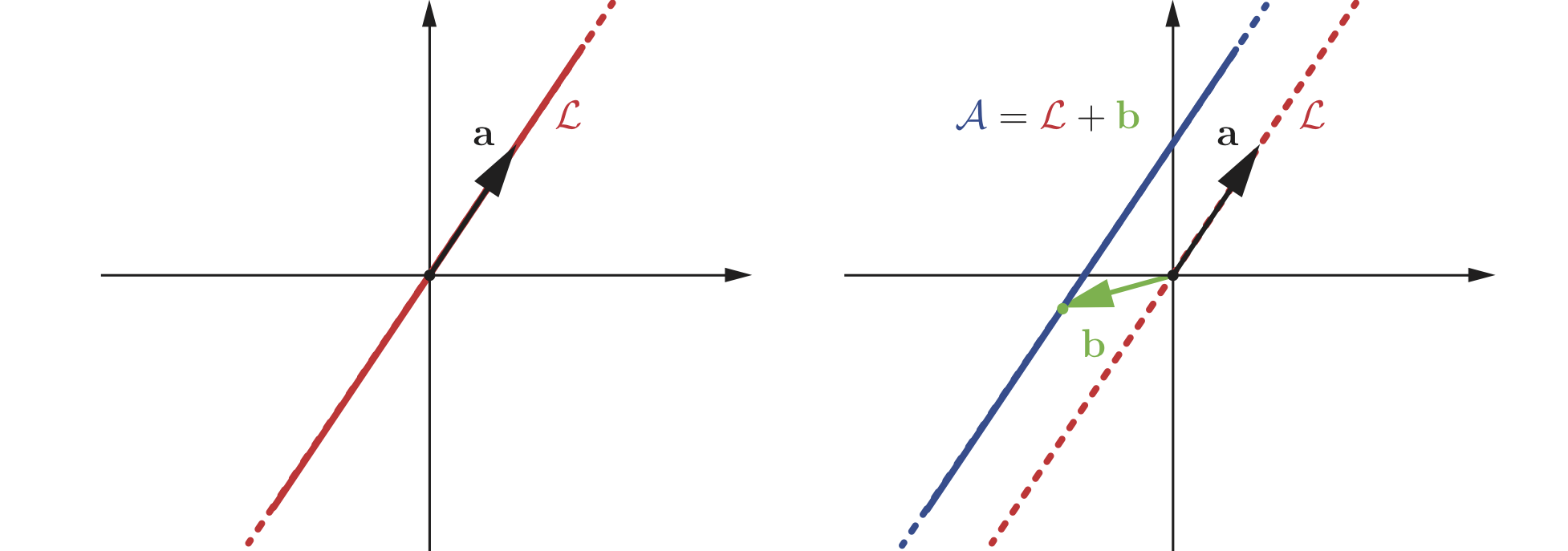
Geometrically, an $m$-dimensional subspace is an $m$-dimensional plane passing through the origin (a one-dimensional plane is a line, a two-dimensional plane is the regular plane, and so on). The latter is true, since setting all the $a_i$’s to zero in the definition of $\mathcal{L}$ yields the zero vector. Figure 1 (left) visualizes this fact.

An affine subspace can be defined as a linear subspace shifted by a vector $\bb{b} \in \RR^n$ away from the origin:

Exercise. Show that any affine subspace can be defined as

The latter linear combination with the scalars restricted to unit sum is called an affine combination.

Vector inner product and norms

Given two vectors $\bb{u}$ and $\bb{v}$ in $\RR^n$, we define their inner (a.k.a. scalar or dot) product as

Though the notion of an inner product is more general than this, we will limit our attention exclusively to this particular case (and its matrix equivalent defined in the sequel). This is sometimes called the standard or the Euclidean inner product. The inner product defines or induces a vector norm

(it is also convenient to write $|\bb{u}|^2 = \bb{u}^\Tr \bb{u}$), which is called the Euclidean or the induced norm.

A more general notion of a norm can be introduced axiomatically. We will say that a non-negative scalar function $| \cdot | : \RR^n \rightarrow \RR_+$ is a norm if it satisfies the following axioms for any scalar $a \in \RR$ and any vectors $\bb{u},\bb{v} \in \RR^n$

1. $|a \bb{u} | = | a | | \bb{u} |$ (this property is called absolute homogeneity);

2. $| \bb{u} + \bb{v} | \le | \bb{u} | + | \bb{v} |$ (this property is called subadditivity, and since a norm induces a metric (distance function), the geometric name for it is triangle inequality);

3. $| \bb{u} | = 0$ iff¹ $\bb{u} = \bb{0}$.

In this course, we will almost exclusively restrict our attention to the following family of norms called the $\ell_p$ norms:

For $1 \le p<\infty$, the $\ell_p$ norm of a vector $\bb{u} \in \RR^n$ is defined as $\| \bb{u} \|_p = \left( \sum_{i=1}^n |u_i|^p \right)^{1/p}.$

Note the sub-index $_p$. The Euclidean norm corresponds to $p=2$ (hence, the alternative name, the $\ell_2$ norm) and, whenever confusion may arise, we will denote it by $| \cdot |_2$.

Another important particular case of the $\ell_p$ family of norms is the $\ell_1$ norm $\| \bb{u} \|_1 = \sum_{i=1}^n |u_i|.$ As we will see, when used to quantify errors for example in a regression or model fitting task, the $\ell_1$ norm (representing mean absolute error) is more robust (i.e., less sensitive to noisy data) than the Euclidean norm (representing mean squared error). The selection of $p=1$ is the smallest among the $\ell_p$ norms for which the norm is convex. In this course, we will dedicate significant attention to this important notion, as convexity will have profound impact on solvability of optimization problems.

Yet another important particular case is the $\ell_\infty$ norm $\| \bb{u} \|_\infty = \max_{i=1,\dots,n} |u_i|.$ The latter can be obtained as the limit of $\ell_p$.

Exercise. Show that $\displaystyle{\lim_{p \rightarrow \infty} \| \bb{u} \|_p = \max_{i=1,\dots,n} |u_i|}$.

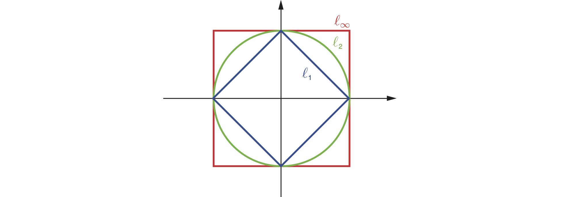
Geometrically, a norm measures the length of a vector; a vector of length $|\bb{u}|=1$ is said to be a unit vector (with respect to² that norm). The collection ${ \bb{u} : | \bb{u} | = 1 }$ of all unit vectors is called the unit circle (see figure). Note that the unit circle is indeed a “circle” only for the Euclidean norm. Similarly, the collection $B_r = { \bb{u} : | \bb{u} | \le r }$ of all vectors with length no bigger than $r$ is called the ball of radius $r$ (w.r.t. a given norm). Again, norm balls are round only for the Euclidean norm. From figure 2 we can deduce that for $p < q$, the $\ell_p$ unit circle is fully contained in the $\ell_q$ unit circle. This means that the $\ell_p$ norm is bigger than the $\ell_q$ norm in the sense that $| \bb{u} |_q \le | \bb{b}|_p$.

Exercise. Show that $| \bb{u} |_q \le | \bb{b}|_p$ for every $p < q$.

Continuing the geometric interpretation, it is worthwhile mentioning several relations between the inner product and the $\ell_2$ norm it induces. The inner product of two ($\ell_2$-) unit vectors measures the cosine of the angle between them or, more generally, $\langle \bb{u}, \bb{v} \rangle = \| \bb{u} \|_2 \| \bb{v} \|_2 \cos \theta,$ where $\theta$ is the angle between $\bb{u}$ and $\bb{v}$. Two vectors satisfying $\langle \bb{u}, \bb{v} \rangle = 0$ are said to be orthogonal (if the vectors are unit, they are also said to be orthonormal) – the algebraic way of saying “perpendicular”.

The following result is doubtlessly the most important inequality in linear algebra (and, perhaps, in mathematics in general):

Theorem: Cauchy-Schwartz inequality. Let $| \cdot |$ be the norm induced by an inner product $\langle \cdot, \cdot \rangle$ on $\RR^n$, Then, for any $\bb{u}, \bb{v} \in \RR^n$,

with equality holding iff $\bb{u}$ and $\bb{v}$ are linearly dependent.

Matrices

A linear map from the $n$-dimensional linear space $\RR^n$ to the $m$-dimensional linear space $\RR^m$ is a function mapping $\bb{u} \in \RR^n$ $\bb{v} \in \RR^m$ according to

The latter can be expressed compactly using the matrix-vector product notation $\bb{v} = \bb{A} \bb{u}$, where $\bb{A}$ is the matrix with the elements $a_{ij}$. In other words, a matrix $\bb{A} \in \RR^{m \times n}$ is a compact way of expressing a linear map between $\RR^m$ and $\RR^n$. An matrix is said to be square of $m=n$; such a matrix defines an operator mapping $\RR^n$ to itself. A symmetric matrix is a square matrix $\bb{A}$ such that $\bb{A}^\Tr = \bb{A}$.

Recollecting our notion of linear combinations and linear subspaces, observe that the vector $\bb{v} = \bb{A}\bb{u}$ is the linear combination of the columns $\bb{a}_1,\dots,\bb{a}_n$ of $\bb{A}$ with the weights $u_1,\dots,u_n$. The linear subspace $\bb{A} \RR^m = { \bb{A} \bb{u} : \bb{u} \in \RR^m \ }$ is called the columns space of $\bb{A}$. The space is $n$-dimensional if the columns are linearly independent; otherwise, if $k$ columns are linearly dependent, the space is $n-k$ dimensional. The latter dimension is called the column rank of the matrix. By transposing the matrix, the row rank can be defined in the same way. The following result is fundamental in linear algebra:

Theorem. The column rank and the row rank of a matrix are always equal.

Exercise. Prove the above theorem.

Since the row and the column ranks of a matrix are equal, we will simply refer to both as the rank, denoting $\rank\, \bb{A}$. A square $n \times n$ matrix is full rank if its rank is $n$, and is rank deficient otherwise. Full rank is a necessary condition for a square matrix to possess an inverse (Reminder: the inverse of a matrix $\bb{A}$ is such a matrix $\bb{B}$ that $\bb{A}\bb{B} = \bb{B}\bb{A} = \bb{I}$; when the inverse exists, the matrix is called invertible and its inverse is denoted by $\bb{A}^{-1}$).

In this course, we will often encounter the trace of a square matrix, which is defined as the sum of its diagonal entries, $\trace\, \bb{A} = \sum_{i=1}^n a_i.$ The following property of the trace will be particularly useful:

Let $\bb{A} \in \RR^{m \times n}$ and $\bb{B} \in \RR^{n \times m}$. Then $\trace(\bb{A}\bb{B}) = \trace(\bb{B}\bb{A})$.

This is in sharp contrast to the result of the product itself, which is generally not commutative.

In particular, the squared norm $| \bb{u} |^2 = \bb{u}^\Tr \bb{u}$ can be written as $\trace(\bb{u}^\Tr \bb{u}) = \trace(\bb{u}\bb{u}^\Tr)$. We will see many cases where such an apparently weird writing is very useful. The above property can be generalized to the product of $k$ matrices $\bb{A}_1 \dots \bb{A}_k$ by saying that $\trace(\bb{A}_1 \dots \bb{A}_k)$ is invariant under a cyclic permutation of the factors as long as their product is defined. For example, $\trace(\bb{A}\bb{B}^\Tr\bb{C}) = \trace(\bb{C}\bb{A}\bb{B}^\Tr) = \trace(\bb{B}^\Tr\bb{C}\bb{A})$ (again, as long as the matrix dimensions are such that the products are defined).

Matrix inner product and norms

The notion of an inner product can be extended to matrices by thinking of an $m \times n$ matrix as of a long vector $m \times n$ vector containing the matrix elements for example, in the column-stack order. We will denote such a vector as $\vec(\bb{A}) = (a_{11},\dots,a_{m1},a_{12},\dots,a_{m2},\dots,a_{1n},\dots,a_{mn})^\Tr$. With such an interpretation, we can define the inner product of two matrices as $\langle \bb{A}, \bb{B} \rangle = \langle \vec(\bb{A}), \vec(\bb{B}) \rangle = \sum_{i,j} a_{ij} b_{ij}.$

Exercise. Show that $\langle \bb{A}, \bb{B} \rangle = \trace( \bb{A}^\Tr \bb{B} )$.

The inner product induces the standard Euclidean norm on the space of column-stack representation of matrices,

known as the Frobenius norm. Using the result of the exercise above, we can write

Note the qualifier $_\mathrm{F}$ used to distinguish this norm from other matrix norm that we will define in the sequel.

There exist another “standard” way of defining matrix norms by thinking of an $m \times n$ matrix $\bb{A}$ as a linear operator mapping between two normed spaces, say, $\bb{A} : (\RR^m,\ell_p) \rightarrow (\RR^n,\ell_q)$. Then, we can define the operator norm measuring the maximum change of length (in the $\ell_q$ sense) of a unit (in the $\ell_p$ sense) vector in the operator domain:

Exercise. Use the axioms of a norm to show that $| \bb{A} |_{p,q}$ is a norm.

Eigendecomposition

Eigendecomposition (a.k.a. eigenvalue decomposition or in some contexts spectral decomposition, from the German eigen for “self”) is doubtlessly the most important and useful forms of matrix factorization. The following discussion will be valid only for square matrices.

Recall that an $n \times n$ matrix $\bb{A}$ represents a linear map on $\RR^n$. In general, the effect of $\bb{A}$ on a vector $\bb{u}$ is a new vector $\bb{v} = \bb{A}\bb{u}$, rotated and elongated or shrunk (and, potentially, reflected). However, there exist vectors which are only elongated or shrunk by $\bb{A}$. Such vectors are called eigenvectors. Formally, an eigenvector of $\bb{A}$ is a non-zero vector $\bb{u}$ satisfying $\bb{A}\bb{u} = \lambda \bb{u}$, with the scalar $\lambda$ (called eigenvalue) measuring the amount of elongation or shrinkage of $\bb{u}$ (if $\lambda < 0$, the vector is reflected). Note that the scale of an eigenvector has no meaning as it appears on both sides of the equation; for this reason, eigenvectors are always normalized (in the $\ell_2$ sense). For reasons not so relevant to our course, the collection of the eigenvalues is called the spectrum of a matrix.

For an $n\times n$ matrix $\bb{A}$ with $n$ linearly independent eigenvectors we can write the following system

Stacking the eigenvectors into the columns of the $n \times n$ matrix $\bb{U} = (\bb{u}_1,\dots,\bb{u}_n)$, and defining the diagonal matrix

we can rewrite the system more compactly as $\bb{A}\bb{U} = \bb{U}\bb{\Lambda}$. Independent eigenvectors means that $\bb{U}$ is invertible, which leads to $\bb{A} = \bb{U}\bb{\Lambda}\bb{U}^{-1}$. Geometrically, eigendecomposition of a matrix can be interpreted as a change of coordinates into a basis, in which the action of a matrix can be described as elongation or shrinkage only (represented by the diagonal matrix $\bb{\Lambda}$).

If the matrix $\bb{A}$ is symmetric, it can be shown that its eigenvectors are orthonormal, i.e., $\langle \bb{u}_i, \bb{u}_j \rangle = \bb{u}_i^\Tr \bb{u}_j = 0$ for every $i \ne j$ and, since the eigenvectors have unit length, $\bb{u}_i^\Tr \bb{u} = 1$. This can be compactly written as $\bb{U}^\Tr \bb{U} = \bb{I}$ or, in other words, $\bb{U}^{-1} = \bb{U}^\Tr$. Matrices satisfying this property are called orthonormal or unitary, and we will say that symmetric matrices admit unitary eigendecomposition $\bb{A} = \bb{U} \bb{\Lambda}\bb{U}^\Tr$.

Exercise. Show that a symmetric matrix admits unitary eigendecomposition $\bb{A} = \bb{U} \bb{\Lambda}\bb{U}^\Tr$.

Finally, we note two very simple but useful facts about eigendecomposition:

• $\displaystyle{\trace\,\bb{A} = \trace(\bb{U}\bb{\Lambda}\bb{U}^{-1}) = \trace(\bb{\Lambda}\bb{U}^{-1}\bb{U}) = \trace\,\bb{\Lambda} = \sum_{i=1}^n \lambda_i}$.

• $\displaystyle{\det\bb{A} = \det\bb{U}\det\bb{\Lambda}\det\bb{U}^{-1} = \det \bb{U} \det \bb{\Lambda} \frac{1}{\det \bb{U}} = \prod_{i=1}^n \lambda_i}$.

In other words, the trace and the determinant of a matrix are given by the sum and the product of its eigenvalues, respectively.

Matrix functions

Eigendecomposition is a very convenient way of performing various matrix operations. For example, if we are given the eigendecomposition of $\bb{A} = \bb{U}\bb{\Lambda}\bb{U}^{-1}$, its inverse can be expressed as $\bb{A}^{-1} = (\bb{U}\bb{\Lambda}\bb{U}^{-1})^{-1} = \bb{U}\bb{\Lambda}^{-1}\bb{U}^{-1}$; however, since $\bb{\Lambda}$ is diagonal, $\bb{\Lambda}^{-1} =\diag{1/\lambda_1,\dots,1/\lambda_n}$. (This does not suggest, of course, that this is the computationally preferred way to invert matrices, as the eigendecomposition itself is a costly operation).

A similar idea can be applied to the square of a matrix: $\bb{A}^2 = \bb{U}\bb{\Lambda}\bb{U}^{-1} \bb{U}\bb{\Lambda}\bb{U}^{-1} = \bb{U}\bb{\Lambda}^2\bb{U}^{-1}$ and, again, we note that $\bb{\Lambda}^2 =\diag{\lambda_1^2,\dots,\lambda_n^2}$. By using induction, we can generalize this result to any integer power $p \ge 0$: $\bb{A}^p = \bb{U}\bb{\Lambda}^p\bb{U}^{-1}$. (Here, if, say, $p=1000$, the computational advantage of using eigendecomposition might be well justified).

Going one step further, let

be a polynomial (either of a finite degree or an infinite series). We can apply this function to a square matrix $\bb{A}$ as follows:

Denoting by $\varphi(\bb{\Lambda}) = \diag{\varphi(\lambda_1),\dots,\varphi(\lambda_n)}$ the diagonal matrix formed by the element-wise application of the scalar function $\varphi$ to the eigenvalues of $\bb{A}$, we can write compactly

Finally, since many functions can be described polynomial series, we can generalize the latter definition to a (more or less) arbitrary scalar function $\varphi$.

The above procedure is a standard way of constructing a matrix function (this term is admittedly confusing, as we will see it assuming another meaning); for example, matrix exponential and logarithm are constructed exactly like this. Note that the construction is sharply different from applying the function $\varphi$ element-wise!

Positive definite matrices

Symmetric square matrices define an important family of functions called quadratic forms that we will encounter very often in this course. Formally, a quadratic form is a scalar function on $\RR^n$ given by $\bb{x}^\Tr \bb{A} \bb{x} = \sum_{i,j=1}^n a_{ij} x_i x_j,$ where $\bb{A}$ is a symmetric $n \times n$ matrix, and $\bb{x} \in \RR^n$.

A symmetric square matrix $\bb{A}$ is called positive definite (denoted as $\bb{A} \succ 0$) iff for every $\bb{x} \ne \bb{0}$, $\bb{x}^\Tr \bb{A} \bb{x} > 0$. The matrix is called positive semi-definite (denoted as $\bb{A} \succeq 0$) if the inequality is weak.

Positive (semi-) definite matrices can be equivalently defined through their eigendecomposition:

Let $\bb{A}$ be a symmetric matrix admitting the eigendecomposition $\bb{A} = \bb{U}\bb{\Lambda}\bb{U}^\Tr$. Then $\bb{A} \succ 0$ iff $\lambda_i > 0$ for $i=1,\dots,n$. Similarly, $\bb{A} \succeq 0$ iff $\lambda_i \ge 0$.

In other words, the matrix is positive (semi-) definite if it has positive (non-negative) spectrum. To get a hint why this is true, consider an arbitrary vector $\bb{x} \ne \bb{0}$, and write

Denoting $\bb{y} = \bb{U}^\Tr \bb{x}$, we have

Since $\bb{U}^\Tr$ is full rank, the vector $\bb{y}$ is also an arbitrary non-zero vector in $\RR^n$ and the only way to make the latter sum always positive is by ensuring that all $\lambda_i$ are positive. The very same reasoning is also true in the opposite direction.

Geometrically, a quadratic form describes a second-order (hence the name quadratic) surface in $\RR^n$, and the eigenvalues of the matrix $\bb{A}$ can be interpreted as the surface curvature. Very informally, if a certain eigenvalue $\lambda_i$ is positive, a small step in the direction of the corresponding eigenvector $\bb{u}_i$ rotates the normal to the surface in the same direction. The surface is said to have positive curvature in that direction. Similarly, a negative eigenvalue corresponds to the normal rotating in the opposite direction of the step (negative curvature). Finally, if $\lambda_i = 0$, a step in the direction of $\bb{u}_i$ leave the normal unchanged (the surface is said to be flat in that direction). A quadratic form created by a positive definite matrix represents a positively curved surface in all directions. Such a surface is cup-shaped (if you can imagine an $n$-dimensional cup) or, formally, is convex; in the sequel, we will see the important consequences this property has on optimization problems.